Stock Market Prediction using News Sentiments- I
An End-to-End Project on Time Series Analysis using Machine Learning.
This is Part-1 of a two-part series.
DISCLAIMER: The information and methods published in this article are solely meant to be used for informational and educational purposes. The contents of this article are not a trading advice and should not be used for real trading practices.

Table of Contents
Part-1
- Introduction
- Why are we using News Sentiments?
- Scoring Metric
- Data Collection
- Data Inspection
- Data Cleaning and Pre-Processing
- Feature Engineering
- Train Test Split
- Exploratory Data Analysis (EDA)
- Making time-series stationary
Part-2
- Modeling
- Anomaly Detection
- Final Model Pipeline for Deployment
- Post-Training Quantization
- Quantized Model Pipeline for Deployment
- Conclusion
- Future Improvements
- Code Reference
- Contact Links
- Papers Referred and Other References
Introduction
Predicting stock market prices has been a topic of interest among both analysts and researchers for a long time. Stock prices are hard to predict because of their high volatile nature which depends on diverse political and economic factors, change of leadership, investor sentiment, and many other factors. Predicting stock prices based on either historical data or textual information alone has proven to be insufficient.
Why are we using News Sentiments?
Market sentiment is a qualitative measure of the attitude and mood of investors to financial markets in general, and specific sectors or assets in particular. Positive and negative sentiment drive price action, and also create trading and investment opportunities for active traders and long-term investors.
Existing studies in sentiment analysis have found that there is a strong correlation between the movement of stock prices and the publication of news articles. Several sentiment analysis studies have been attempted at various levels using algorithms such as Support Vector Machines, Naive Bayes Regression, and deep learning. The accuracy of deep learning algorithms depends upon the amount of training data provided.
Scoring Metric
Since it is a regression problem and the price values of the index are higher, we will use Root Mean Square Error (RMSE) to compare the performance of various models.
Data Collection
We are using the Nifty 50 Index for the stock price data and Stock News from a popular twitter handle.
Nifty 50 Index Data
The historical data of Nifty 50 Stock Price for the last 20 years i.e. from 01/01/2000 to 31/12/2019 was scraped using BeautifulSoup from investing.com.
Twitter News Data
Tweets from popular news handle @NDTVProfit were collected using Twint Scraper Library. Historical data for the last 5 years i.e. from 01/01/2015 to 31/12/2019 was collected.
Data Inspection
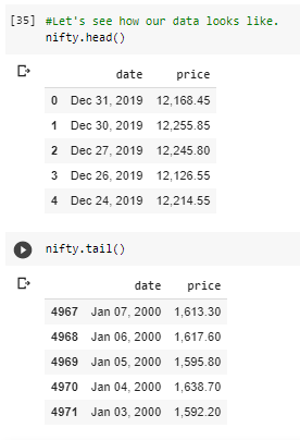
Nifty 50 Index Data
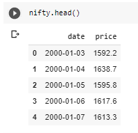
This data contains stock prices corresponding to each day whenever the stock market was functional. We have data for the last 4972 dates and the closing Nifty 50 Index Stock Price for that day.
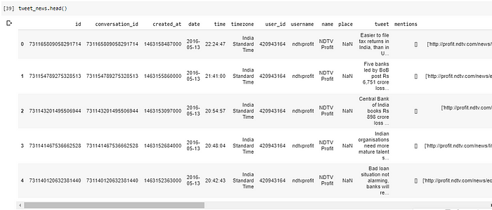
Twitter News Data
This data contains all the tweets which NDTV Profit tweeted in the last 5 years. We have 64,278 tweets data. There is a lot more extra information present for each tweet like username, URL, photos, mentions, likes, retweets. But in this case study, we will focus on only dates and the tweets tweeted on that day.
Data Cleaning & Pre-Processing
Nifty 50 Index Data
The date column is not in proper DateTime datatype and prices contain ‘,’ in-between we need to remove them to consider prices as numerical numbers.
Let’s fix these problems.
Twitter News Data
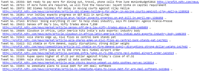
Twitter is a social media and formal language is often ignored. However, since its a news channel so we are expecting the tweets to be written in a formal language.
Some Raw Tweets after Scraping:
We need to perform the following operations on the tweets in order to clean them:
- Convert them into lowercase.
- Remove all the links starting with either http or pic.twitter.com or https
- Remove all the special characters, emoticons
- Remove all the hashtags (#), @ symbol.
- Remove these words: ETMarkets, ndtv, moneycontrol, marketsupdate, biznews, NewsAlert, Click here for LIVE updates.
- Remove all the numbers.
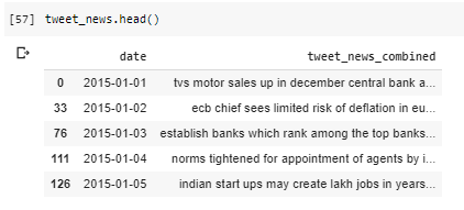
After cleaning we need to combine all the tweets in a single paragraph for each day.
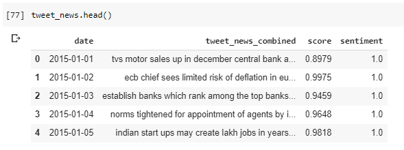
After all the cleaning and pre-processing our data looks like this:
Feature Engineering
We have not tokenized, removed stopwords, and got bigrams, etc because we will be using a pre-trained sentiment analyzer VADER here since our data is unsupervised. We are choosing VADER here because it works very well especially with social media text.
VADER gives a compound score for each paragraph. Score = -1 signifies negative news and score = 1 signifies positive news. Positive news should raise the index prices and vice versa.
Train Test Split
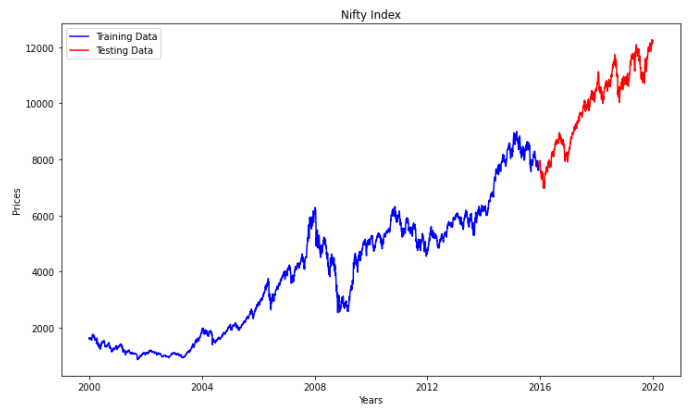
Since it is a time-series data we cannot split it randomly. Hence, we are considering the latest 20% data as a test set and the first 80% data as a train set. Train Data Shape: (3977, 2), Test Data Shape: (995, 2)
Exploratory Data Analysis (EDA)
Exploratory Data Analysis is the process of exploring data, generating insights, testing hypotheses, checking assumptions, and revealing underlying hidden patterns in the data.
Twitter News Data
Checking for Missing Data
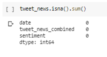
We do not have any missing data here.
Checking for Duplicate Rows
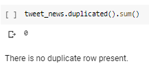
We do not have any duplicate data here.
Sentiments Distribution
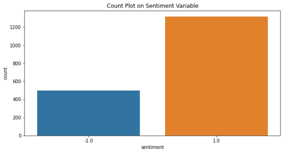
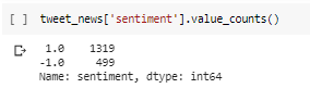
Here, Sentiment = 1: Positive News and Sentiment = -1: Negative News.
We can observe a more number of positive news which reflects why nifty shows an upward trend overall. We have 38% negative tweets here. The results are looking realistic so far.
Word Clouds
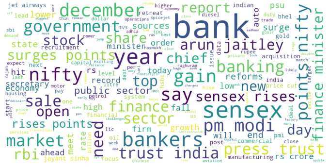
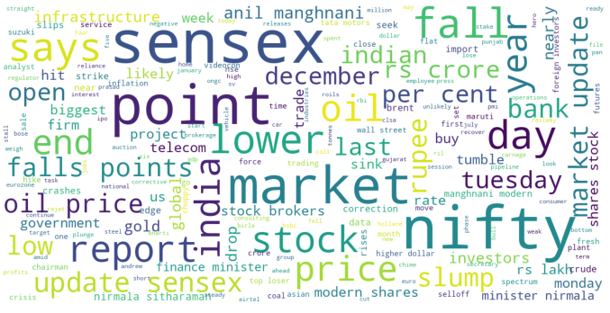
We can observe that words like gain, top, rise, surge result in a positive tweet, and words like lower, fall, hit, drop, slump result in a negative tweet. Looks like bank stocks are the most fluctuating ones.
Probability Distribution of Sentiment Scores by VADER
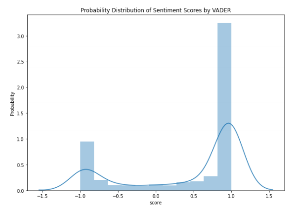
For the majority of news, VADER is confident in detecting either positive or negative sentiment since most of the points lie on the boundary. This shows accurate and confident prediction from VADER library
Date-wise Distribution of News Sentiments
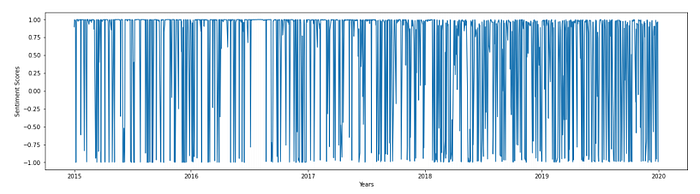
We can observe that we had more positive news before 2018 than after 2018. The number of news also increased as we move towards 2020.
Nifty 50 Index Data
Checking for Missing Data
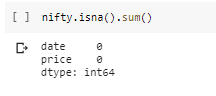
We do not have any missing data here.
Checking for Duplicate Rows
We do not have any duplicate data here.
Probability Distribution of Nifty index Closing Prices
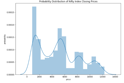
Nifty index price hovered over 1000 and 5000 levels for the most time in the past 20 years. It rarely went past 13000 levels.
Stationarity of a Time Series
There are three basic criteria for a time series to understand whether it is a stationary series or not. Statistical properties of time series such as mean and variance should remain constant over time to call time series stationary.
Following are the 3 qualities of a stationary time series:
- Constant mean
- Constant variance
- Autocovariance that does not depend on time. Autocovariance is the covariance between the time series and lagged time series.
Let’s visualize and check the seasonality and trend of our time series first.
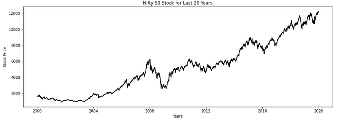
Trend: This time series shows an upward trend. This is a non-stationary time series. We need to convert it to stationary to forecast accurately. Let’s also check for seasonality.
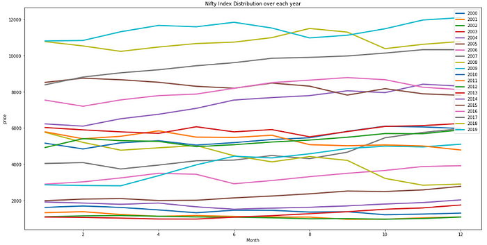
Seasonality: The time series has a slight seasonal variation.
We can observe a decline in prices in the latter half of the year. From January to June months we can see a general upward trend. The first 6 months are relatively safer for investing and one should sell by June or July month.
If one observes a downward trend in the graph for the first 6 months of the year then chances are that it will continue to drop further in the next 6 months. So one should sell as soon as possible in this case or keep holding the stock for a longer period.
Now let’s check the stationarity of time series. It can be checked using the following methods:
- Plotting Rolling Statistics: We have a window lets say window size is 6 and then we find rolling mean and variance to check stationary.
- Dickey-Fuller Test: The test results comprise a Test Statistic and some Critical Values for different confidence levels. If the test statistic is less than the critical value, we can say that the time series is stationary.
We will use hypothesis testing here.
We state Null Hypothesis here that time series has a unit root which means it is non-stationary. And an Alternative Hypothesis that time series is stationary.
For time series to be stationary we should get a p-value of less than 5% to reject the null hypothesis.
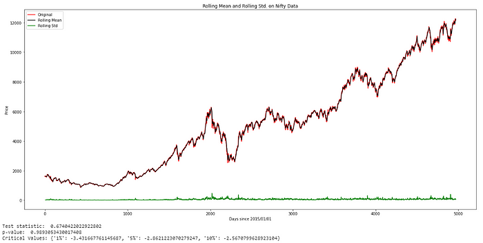
a. Our first criterion for stationary is a constant mean. So we fail because mean is not constant as you can see from the plot (black line) above.
b. The second one is a constant variance. It looks like constant. (Green Graph above)
c. The third one is that if the test statistic is less than the critical value then we can say that time series is stationary.
Lets look: test statistic = 0.674 and critical values = {‘1%’: -3.431667761145687, ‘5%’: -2.8621223070279247, ‘10%’: -2.5670799628923104}.
The test statistic is bigger than the critical values. So, no stationary.
As a result, we are sure that our time series is not stationary. Let's make time-series stationery in the next part.
Two methods which can help us make it stationary:
- Moving Average Method
- Differencing Method
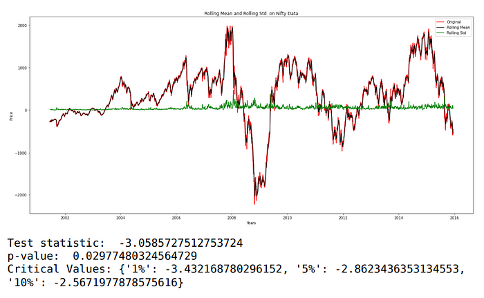
Mean is constant over time. There is no trend visible, the p-value is also less than 5%. But the test statistic is not less than Critical Value. Variance is not constant. Our time series is still not stationary.
Let’s try the differencing method.
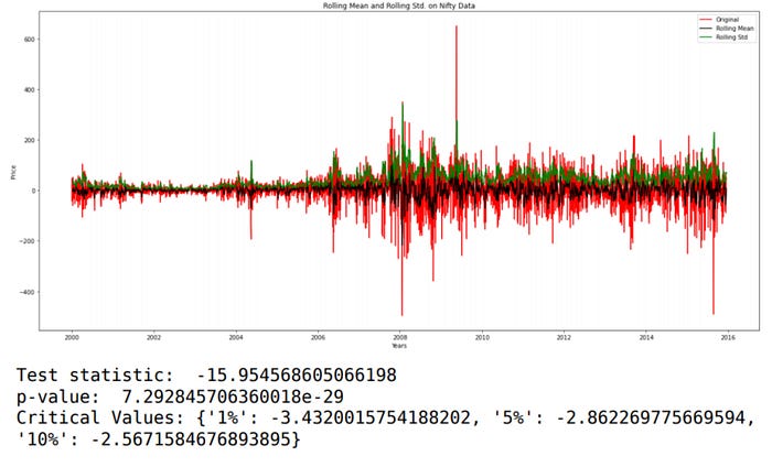
Much better results! Differencing method wins here because it is producing more stationary time series than the moving average method as Test Statistic is lesser in case of differencing method.
We will be using this stationary time series for forecasting. STAY TUNED!
Link to Part-2 of this blog: https://medium.com/@kala.shagun/stock-market-prediction-using-news-sentiments-dc4c24c976f7
Code Reference
Contact Links
Email Id: kala.shagun@gmail.com
Linkedin: https://www.linkedin.com/in/shagun-kala-061a3b127/
Papers Referred
- Stock Price Prediction Using News Sentiment Analysis: http://davidanastasiu.net/pdf/papers/2019-MohanMSVA-BDS-stock.pdf
- Sentiment Analysis of Twitter Data for Predicting Stock Market Movements: http://arxiv.org/pdf/1610.09225v1.pdf
Other References
- AppliedAICourse.com
- www.tensorflow.org/lite/performance/post_training_quantization
- https://github.com/sonalimedani/TF_Quantization/blob/master/quantization.ipynb
- https://towardsdatascience.com/end-to-end-time-series-analysis-and-modelling-8c34f09a3014
- https://medium.com/analytics-vidhya/stock-prices-prediction-using-machine-learning-and-deep-learning-techniques-with-python-codes-a630c0d3f137
- https://udibhaskar.github.io/practical-ml/debugging%20nn/neural%20network/overfit/underfit/2020/02/03/Effective_Training_and_Debugging_of_a_Neural_Networks.html
- https://machinelearningmastery.com/how-to-develop-lstm-models-for-time-series-forecasting/